
where delays are shown to be counterintuitive.
Leaving the house (and the country) for a week or two during the holiday season is a great time to get out of my stereotypical ways of passing free time (entirely too much YouTube, Lobste.rs, HackerNews and BlueSky) and try something else.
For my recent vacation I have packed some grid paper to make a bitmap font, and two books: the first one was Nachové pustiny: a Czech post-apocalyptic novel to get some inspiration for my “Fallout but in Czech Republic” MMO game, and the other was Thinking in Systems: a book recommended at work (and bought with my work education budget) which was collecting dust in my bookshelf for a good few months now.
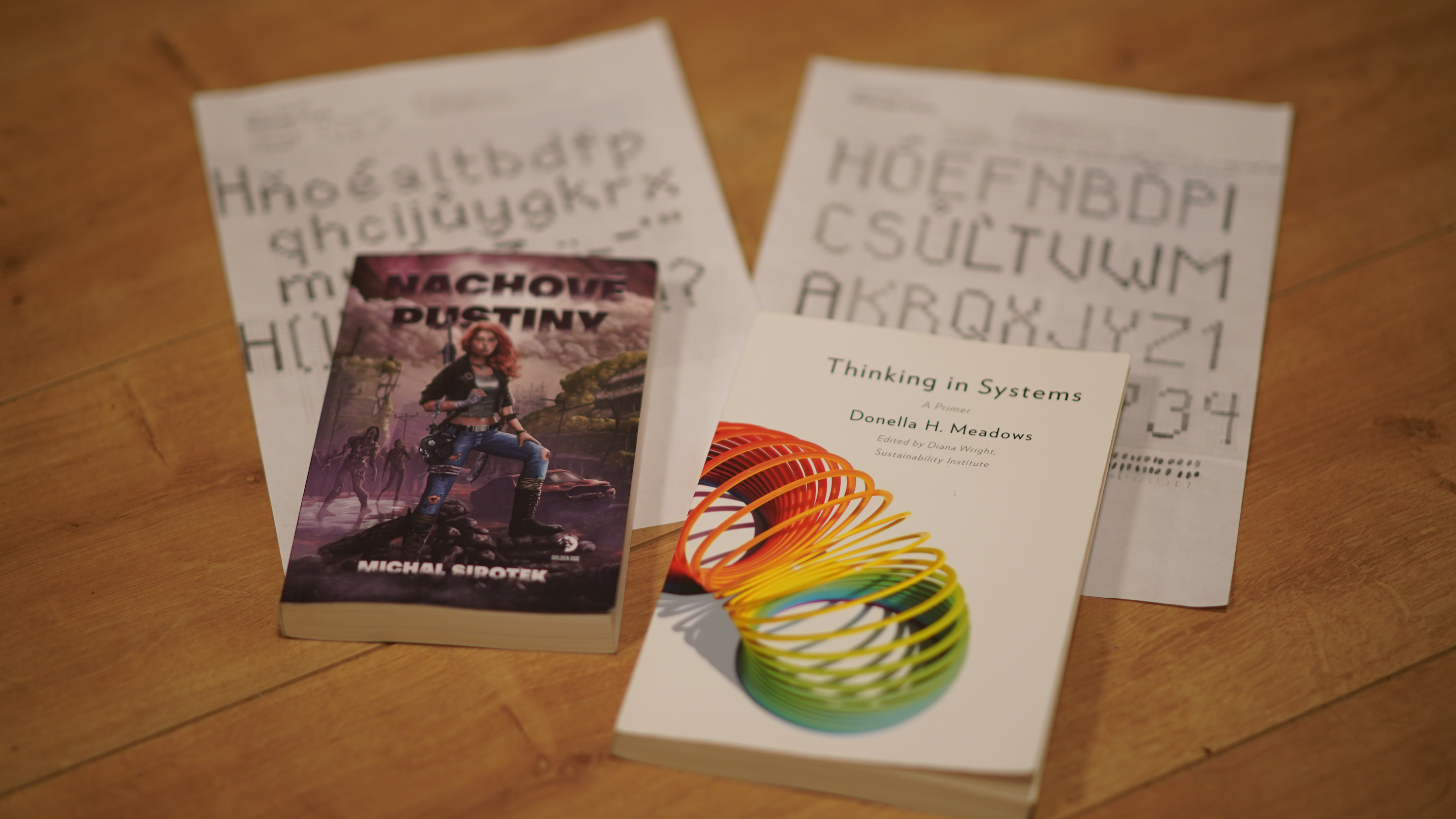
I’m happy to announce I managed to get through all three of these goals: I’ve created a bitmap font (though I still have kerning and accents to go through), devoured the post-apo novel (it was okay), and got through the systems book!
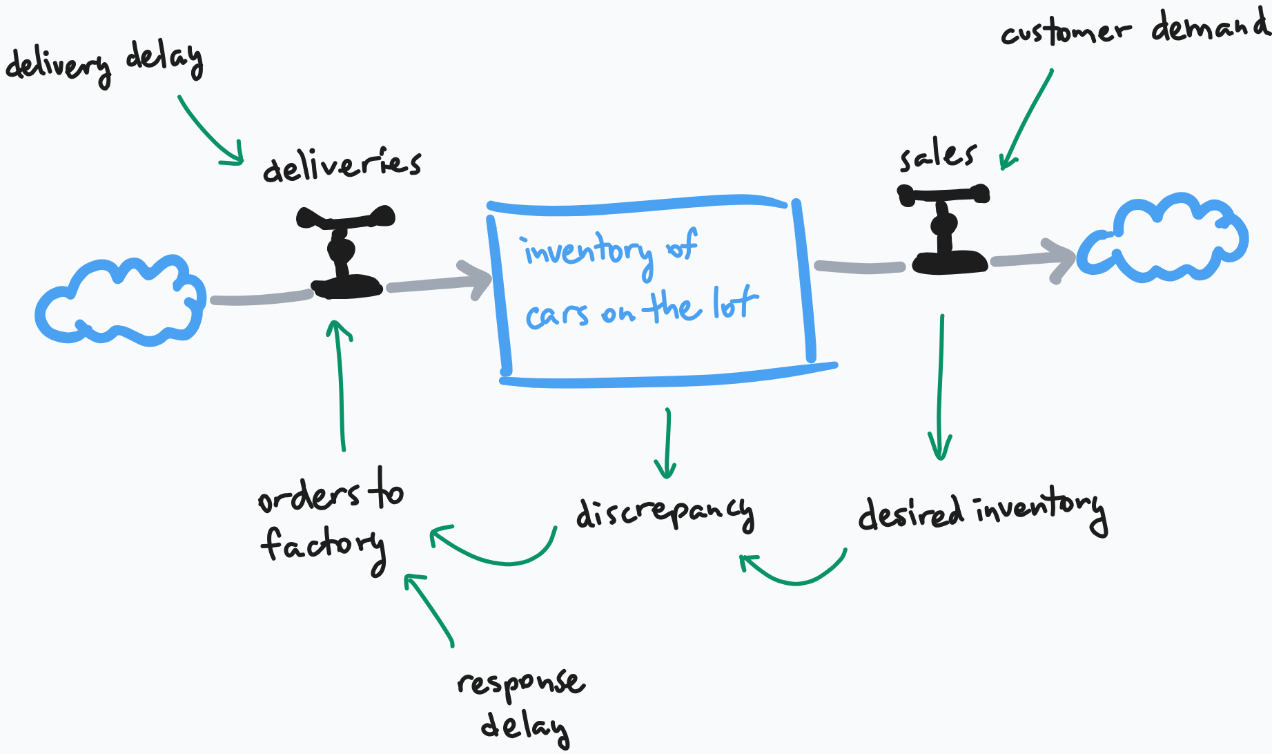
Thinking in Systems introduces a framework and a visual language of sources and sinks, stocks and flows, feedback loops and systems that (more often than not) emerge bottom-up from them.
It all roughly corresponds to mathematical models and differential equations, though the book doesn’t go into detail of those and only mentions the actual formulas for its examples in an appendix.
Delays are weird
There was one really cool chapter that IMHO is the highlight of the whole book. It concerns delays.
The running example (see image above) is a car dealership manager shepherding a stock of cars on their parking lot, aiming for it to always be 10x the amount of cars sold. When the customer demand rises, she starts ordering more cars to cover the gap.
Delay-less system
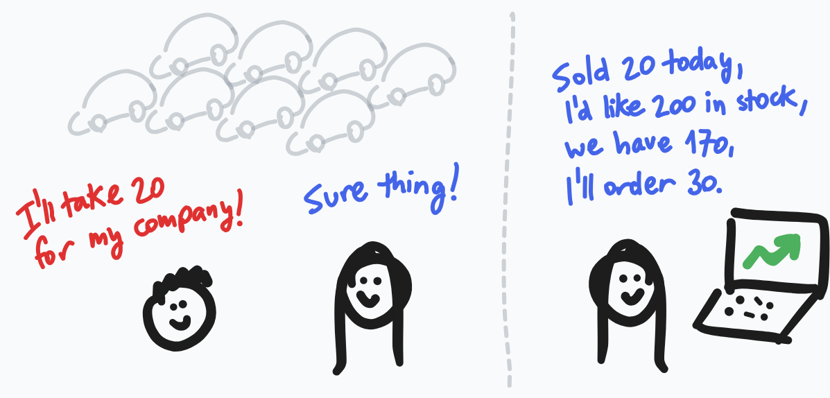
In an ideal world there are no delays: she immediately sees an increased demand and the discrepancy between the current stock and the ideal one, she immediately sends an order to bring more cars in, and the cars immediatelly arrive.
Also, in this example the time granularity is days, so imagine that at the end of the day she sees 30 cars got sold, sends an order for 30 cars and they arrive the next morning.
Let’s first see the constants in our model that won’t be affected by the delays:
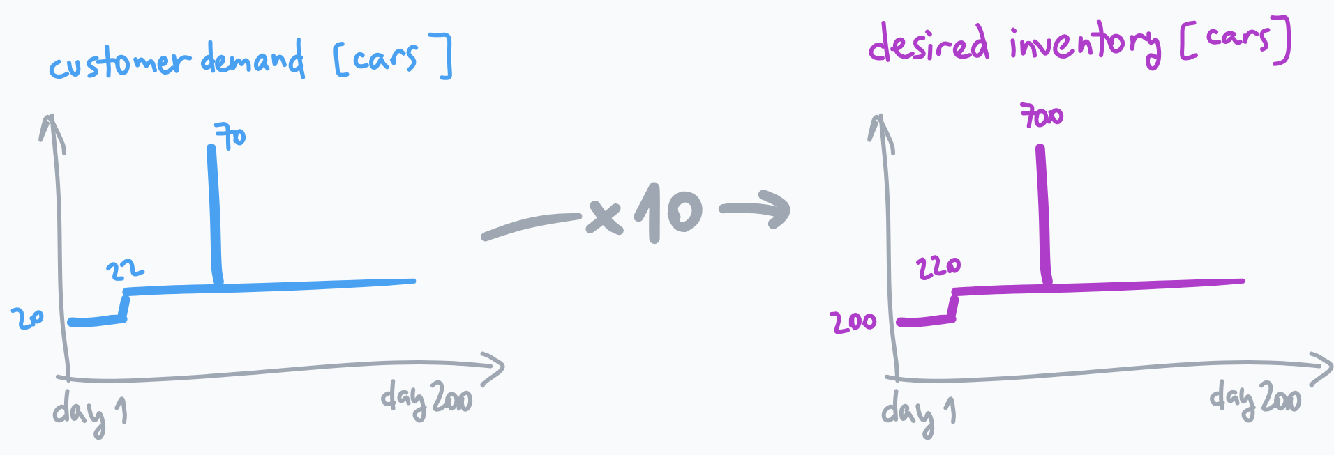
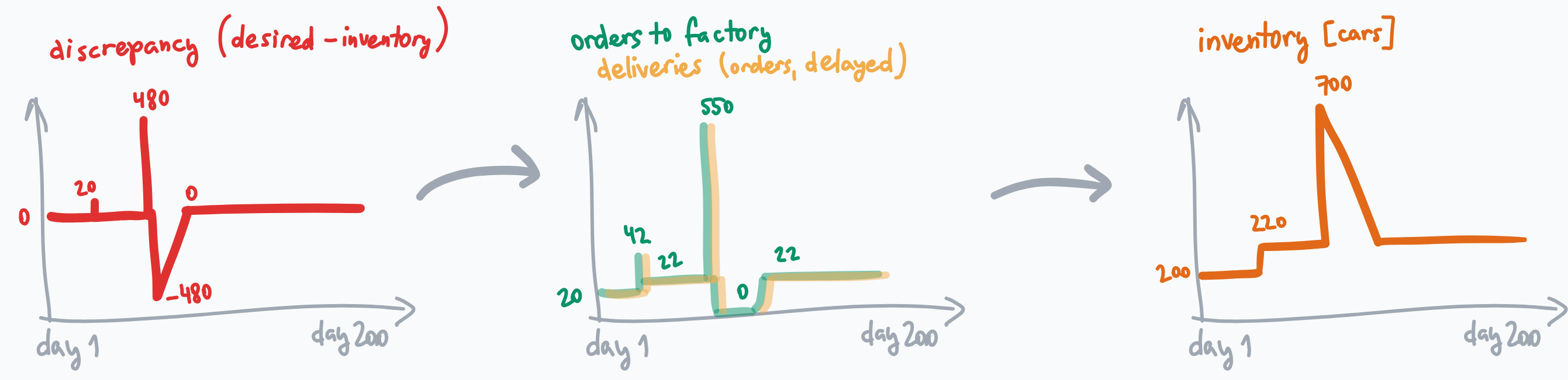
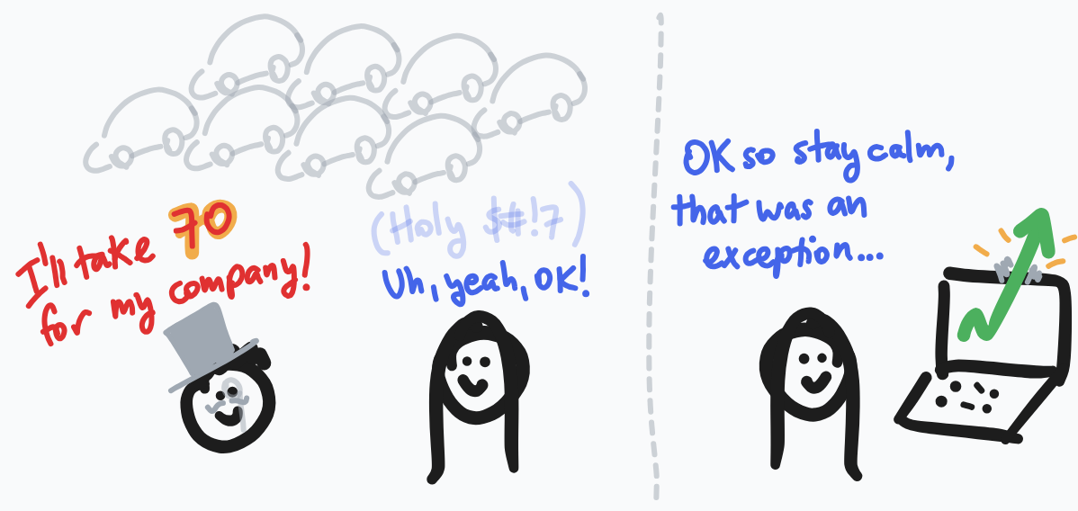
The customer demand starts at 20 cars each day, then ramps up to 22 cars each day, with a spike of 70 cars on one specific day.
Sales are min(customer demand, inventory), which in all examples below will equal customer demand, as we have enough cars ready, but you can imagine getting out of stock if demand gets high enough fast enough.
Our manager calculates the desired inventory as sales * 10. Might be simplistic but hey, it’s an example.
You could also imagine us later averaging over sales from past N days and basing the desired inventory off of that, and thus introducing yet another delay into the system, but I’ve omitted it from this blogpost as it doesn’t touch what I want to illustrate.
So, how does the delay-less model behave?
BTW, I have written a Monte Carlo simulator myself in Elm while reading the book—it lists the pseudocode formulas for the examples in this blogpost—but a spreadsheet would suffice, and there are other tools to deal with these differential equation models. Heck, there’s a free graphical webapp built on top of a JS library showing off the same example I do in one of its examples. I guess the book is influential.
This model has no delays, but it has an issue with overreacting to the random spikes in customer demand by buying too many cars which then take forever to sell, and more importantly it’s unrealistic: in the real world everything has a bit of a delay. The orders take time to process, the cars take time to arrive at the dealership lot, and so on. We’ll call that the delivery delay.

That seems like a bad delay, but delays don’t need to always be bad: consider that the manager might want to not overreact to those random spikes. She had ordered 550 cars because of a spike, when she normally orders only around 20 a day! Instead she might want to get to the desired inventory slowly over time by ordering only half of the discrepancy, or a third, etc. If on the next day things get back to normal, we’ll be able to ride the wave much more smoothly without overreacting. Let’s call this divisor the response delay.
System with delays
Let’s run the model with these two delays and see:
- delivery delay: 5 days (from me sending the order to the cars arriving on the lot)
- response delay divisor: 2 (if I see a discrepancy of 30 cars, I’ll only order 15 today.)
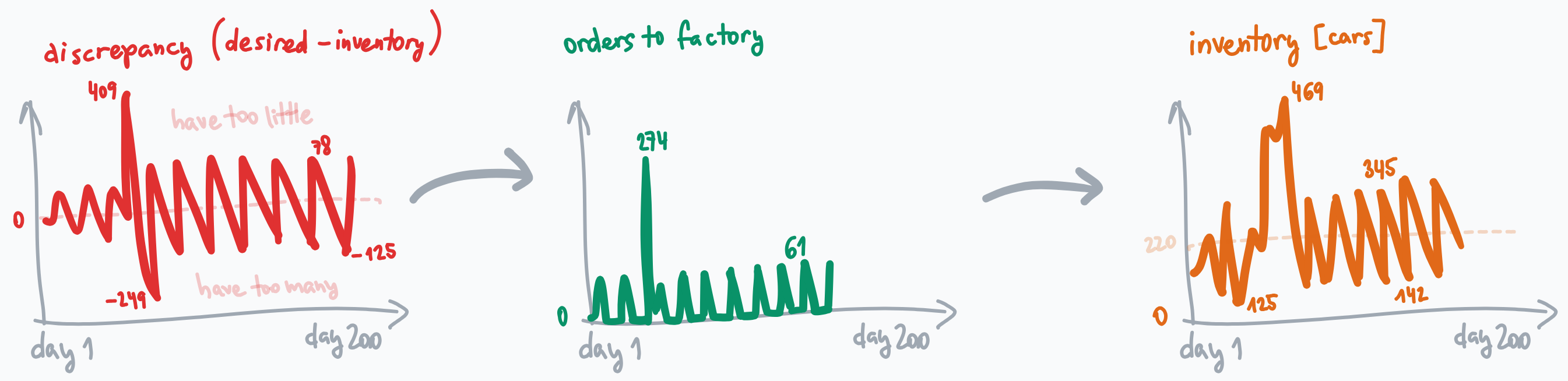
What? What just happened? We thought we’re doing everything right, the response delay was a good thing!
Well it is. But the combination of the two delays made our system oscillate! It never stabilizes even if the customer demand remains constant afterwards.
The manager is caught in a vile cycle of ordering too many cars, then ordering more and more the following days before the first order arrives. Once orders start arriving, she now has too many cars and ends up not ordering any more while waiting for the inventory to get back to the ideal levels. But then with more car sales the inventory dips below the ideal again and she starts the cycle again.
I’d be interested in learning what, mathematically, makes these oscillations inevitable. Some more math-heavy book on these models and differential equations will probably explain that. For now let’s just take the oscillations caused by delays for a fact.
Shorter delays: surely the fix?
Now you might think that since delays got us into this mess, we should minimize them as much as possible. Shorten the feedback loop and all. But remember, we introduced the response delay to be more resilient towards random spikes. Anyways, let’s try and see what happens:
- delivery delay: 5 days (we can’t speed up this one)
- response delay divisor: 1 (be as fast as we can: buy the exact amount we’re missing at end of day)
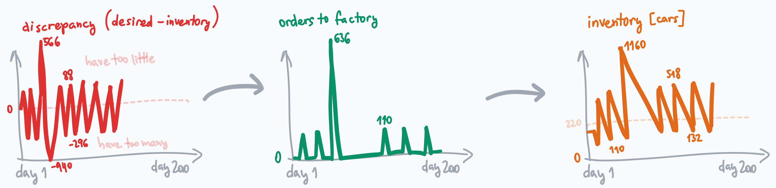
Hm. As you can see, trying to be faster made things worse: our inventory of cars now oscillates much more: cycles of shooting up from 132 to 518, while we’d like to be around 220. Not to mention having to have 1160 cars in our lot at once after the spike! This is even worse than the no-delays scenario! Is there any hope?
Longer delays: Take it easy, Dude…
Just to see what will happen: let’s simulate a more patient manager: one that spreads out the restocking over a longer period of time. Let’s make our response delay divisor larger and try 6. When we see a discrepancy of 30 cars at the end of the day, let’s just order 5 instead of 10 or 15 or 30.
- delivery delay: 5 days (still out of our control)
- response delay divisor: 6 (slower response! longer delay!)
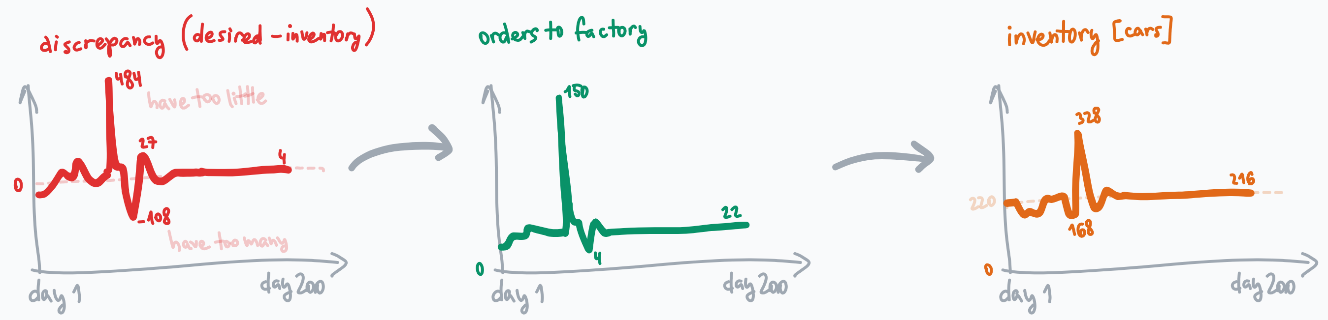
Wow! The oscillations died out and stabilized!
Conclusion
This was pretty counterintuitive to me when I read it. Delays intuitively seem like something you want to minimize. But here, shortening a delay made things worse and making it longer made things more predictable and less wasteful.
In the later parts of the book Donella Meadows mentions short feedback loops; there’s no clear cut rule that you could apply blindly. Make a model of your system, try different parameters, see how it behaves.
Many managers and leaders take the lever that the researchers provide, and crank it full speed, wrong direction. You might think you know which way is the correct one, but maybe, just maybe, get insight into how your system would behave in both directions and act on data instead of on intuition.
P.S.
Feel free to play around with the toy simulator for this example. The code is at Github.